SQL Server Execution Plans: A DBA’s Triage Guide

SQL Server Execution Plans: A DBA’s Guide to Reading and Fixing Them

Generating a SQL Server execution plan is the easy part. 

You pull it up in SSMS and view a graph of operators and arrows that the documentation taught you to produce, but never quite taught you to read.

Most of us fall into the same habit, scanning left to right, settling on whichever operator carries the highest cost percentage, and tuning that.

The instinct is reasonable. The catch is that the expensive-looking operator is usually downstream of the real problem, grinding through rows that a poor access method or join choice upstream produced.

Tune it, and you’ve treated a symptom while the upstream issue keeps producing those rows. The real fix is often upstream, closer to the operators that produced those rows in the first place. Once the access path, join choice, or estimate problem is addressed, the expensive-looking operator often settles on its own.

This guide assumes you can already tell a seek from a scan, so it skips the primer and works through triage instead: a repeatable way to get from an open plan to a diagnosed cause and a fix that holds. The harder question usually arrives earlier, before any plan is even open: which of a few hundred active queries is the one worth opening?

Key takeaways

• The most expensive-looking operator is usually a symptom, not the cause. Follow the thickest arrow to where row counts blow up, because that high-cost operator is often just dutifully processing the excess rows, a bad access method, or a join upstream already produced.
• Right-click the operator and open Properties, not the tooltip, then compare Estimated Number of Rows against Actual Number of Rows. That one comparison drives nearly every decision that follows, since a wide gap means the plan was built for a workload your database isn’t actually running.
• Bad cardinality estimates underlie most poor plans, and stale statistics are the usual culprit. When estimated and actual rows diverge, check the currency with DBCC SHOW_STATISTICS and STATS_DATE before you touch indexes or rewrite anything.
• When you spot a Key Lookup, add INCLUDE columns to the index already doing the Seek rather than spinning up a fresh covering index. A net-new index costs you write latency on every insert, update, and delete, and that bill grows with every redundant index you add to dodge a lookup.
• The plan cache only shows what’s running right now and keeps no history. “It was fast yesterday.” Problems belong in Query Store, where the Regressed Queries report puts the before-and-after plans side by side. The harder question is which of your hundreds of active queries to open first, which is where a monitoring layer earns its place.

How SQL Server execution plans flow and where most DBAs look first

It helps to be precise about what you’re looking at first. An execution plan is the blueprint that the optimizer commits to for a single query, the specific set of physical operations it chooses to fetch, join, sort, and return your rows. Each box is an operator, one discrete step such as a seek, a scan, or a join. The arrows between them carry the rows passed from one step to the next. Put together, the plan is the engine showing its work, and the rest of this section is about reading that work in the right order.

Plans read right-to-left, but experienced developers still scan left-to-right. 

The rightmost node is the first data source SQL Server touches; the leftmost is the final output. Everyone learns this and forgets it under pressure, defaulting to the SELECT or the first operator they recognize. 

That instinct is misleading because the high-percentage operator on the left is often downstream of the real problem, dutifully processing the excess rows that a poor upstream access method or join strategy has already produced. Fix the upstream cause, and the expensive-looking operator stops being expensive.

The correct first-triage sequence starts with the thickest arrow. 

Arrow thickness represents the row volume flowing between operators, so the fattest arrow points to where the largest row-count discrepancy lives. The sequence is straightforward. Find that arrow, right-click the operator feeding it, and open Properties rather than the tooltip, since the tooltip rounds and truncates while the Properties pane shows exact values. 

Then compare the Estimated Number of Rows against the Actual Number of Rows. That single comparison drives every decision that follows. Operator-level CPU and elapsed time are also available in Properties on SQL Server 2014 and later, and for queries that run long enough to make waiting for an actual plan impractical, Live Query Statistics animates the flow in real time.

Why cardinality estimation is where most execution plans fail

Cardinality estimation is the optimizer’s prediction of how many rows each operator will process, and when it’s wrong, every downstream decision is wrong. 

The query optimizer does not pick between a Nested Loops join and a Hash Match at runtime based on real data. It builds the plan during compilation, using statistics (histograms stored per column) to estimate how many rows each operator will handle. 

When those estimates hold, the optimizer generally chooses well. When they’re badly off, the plan is engineered for a problem the database isn’t actually solving: Nested Loops chosen for a workload that needs Hash Match, a 4 MB memory grant on a query that spills gigabytes to tempdb, an Index Seek that collapses into a Table Scan because selectivity was underestimated. The individual operators get blamed, but the root cause is almost always the estimate behind them.

Multi-column predicates with correlated columns are where cardinality estimation breaks down the most.

By default, the estimator assumes column independence, calculating the selectivity for each column and then multiplying them. On a table where State = ‘TX’ returns 25% of rows and City = ‘Houston’ returns 2%, the model estimates the combined predicate at 0.5%. But if most Houston customers are also in Texas, the actual selectivity is closer to 2%, and that gap is exactly the estimated-versus-actual divergence you spotted in the Properties pane. 

It’s the signal that should prompt you to check the currency statistics. This matters for teams that have seen regressions after a version upgrade. SQL Server 2022 ships an updated cardinality estimator, and raising the database compatibility level changes which CE version the optimizer uses, which can shift plan choices on queries that ran fine for years.

The practical check is DBCC SHOW_STATISTICS against the query’s predicate columns. When the row-count gap is large, verify whether the histogram still reflects reality. DBCC SHOW_STATISTICS (‘TableName’, ‘IndexOrStatisticName’) returns the histogram directly, and STATS_DATE() tells you when it was last updated. Compare that date with the volume of changes since then. 

On SQL Server 2014 and earlier, auto-update doesn’t trigger until 20% of rows have changed, so on a 100-million-row table, statistics can be months old before SQL Server automatically refreshes them. SQL Server 2016 and later apply a more aggressive dynamic threshold for large tables, but manual update schedules for heavily loaded OLTP tables remain a common gap. Running UPDATE STATISTICS and re-checking the plan is the fastest way to confirm whether stale statistics are the culprit.

The key lookup fix most DBAs get wrong

The NonClustered Index Seek to Key Lookup to Nested Loops pattern is one of the most recognizable in any plan, and it has a specific cause. 

The nonclustered index found the qualifying rows (the Seek), but it doesn’t contain every column the SELECT clause needs, so SQL Server returns to the clustered index or heap to fetch the rest. That’s the Key Lookup, and Nested Loops drives the repetition: one lookup per row the Seek returned. At scale, this compounds fast. A query executing thousands of times an hour, returning 500 rows per call, fires 500 lookups per execution, and when each is a random I/O against a large clustered index, the cumulative cost is brutal. SSMS flags it for you with a green missing-index hint on the operator once the lookup count reaches a high enough threshold.

The correct fix is to include columns on the existing index. 

The common reflex is to create a fresh index that covers the SELECT columns. The better move is adding INCLUDE columns to the index already doing the Seek, like CREATE INDEX IX_ExistingName ON dbo. Table (KeyCol) INCLUDE (Col1, Col2, Col3). INCLUDE columns carry no key-size overhead, don’t disturb the sort order the Seek depends on, and spare you the maintenance cost of a net-new index. That cost is the real reason the wrong fix hurts. An OLTP database with index sprawl incurs write latency on every INSERT, UPDATE, and DELETE across all indexes, and the bill grows with every redundant index you add to dodge a lookup.

Query Store and catching plan regressions before users do

sys.dm_exec_cached_plans only shows the plan SQL Server is currently using. Query Store shows what changed and when. 

Plan cache inspection is a snapshot. 

The cache evicts under memory pressure, overwrites on recompile, and keeps no history, so when you investigate “it was fast yesterday,” yesterday’s fast plan may already be gone. Query Store, enabled by default in SQL Server 2022 and available since 2016, stores the full plan history per query: every plan that ran, when it ran, its cost, and whether a plan change tracked with a performance change. The Regressed Queries report puts the before-and-after plans side by side, making it the correct starting point for regression work. sys.dm_exec_query_stats can surface currently expensive queries, but it can’t reconstruct the history that explains why they got that way.

Parameter Sensitive Plan optimization in SQL Server 2022 addresses a class of parameter-sniffing failures that Query Store alone can’t fix. 

Classic sniffing happens when SQL Server caches a plan compiled for one parameter value that then runs catastrophically for another, like a plan tuned for a customer with 10 million orders being reused for one with 10. 

PSP optimization, at database compatibility level 160, lets the optimizer generate multiple plan variants for a single query, each suited to a different parameter range. It doesn’t require a new server version, only raising the compatibility level. Teams running SQL Server 2019 or 2022 who haven’t moved to level 160 are leaving this improvement on the table.

How IDERA SQL Diagnostic Manager changes the execution plan workflow

• The bottleneck in execution plan analysis is knowing which of your hundreds of active queries to open first.
  A DBA who can diagnose a cardinality failure, fix a key lookup, and read the Regressed Queries report still needs a place to begin. Manually correlating DMV output across a busy production instance to find the queries most likely to carry bad plans is itself slow work. The plan cache ranks queries by resource consumption, which is a consequence rather than a cause. A high-CPU query might have a flawless plan and simply receive heavy traffic, while a query with a brutal Key Lookup storm might run infrequently enough to stay below the top-DMV threshold entirely.
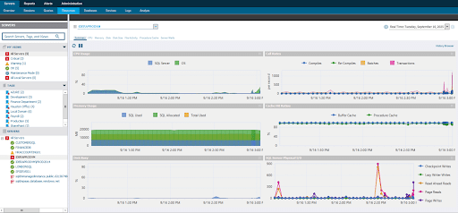
• IDERA SQL Diagnostic Manager identifies top resource-consuming queries, surfaces their execution plans inside the monitoring interface, and ties plan data to the wait statistics and blocking context that explain the slowdown.
  Instead of opening SSMS and scanning plan cache by hand, IDERA SQL Diagnostic Manager alerts on queries that cross configurable thresholds for CPU, duration, or logical reads, then presents the plan alongside that query’s historical baseline. You arrive at the plan already knowing it’s a regression, already seeing which wait types are piling up, already holding the baseline for comparison. IDERA SQL Diagnostic Manager monitors all instances from a single console, which matters when the manual DMV-to-cache workflow doesn’t scale across dozens of servers. It doesn’t replace the analytical skills in this guide. It removes the time spent finding the right query to apply them to.

Getting proactive about execution plan analysis

Reactive analysis (triggered by a user complaint or a ticket that arrived after the damage was done) is the expensive way to work. 

The triage sequence, the cardinality checks, the key lookup remediation, and the Query Store regression hunt all pay off most when you run them before users feel the impact. The two halves of the job, knowing how to read a plan and knowing which plan to read, only close the loop together. 

Start your free trial of IDERA SQL Diagnostic Manager and get the visibility that points you at the bad plan before a support ticket does.

Frequently Asked Questions About SQL Server Execution Plans

What is the difference between an estimated and an actual execution plan in SQL Server? An estimated plan is generated without running the query, showing what the optimizer intends to do based on statistics, with zero I/O. An actual plan captures runtime row counts, memory grant usage, and tempdb spills, showing what SQL Server really did. Start with the estimated plan, then capture an actual plan in a non-production environment, matching production data volume when the estimated counts suggest a statistics problem.

How do I find which queries have bad execution plans in SQL Server? Two primary methods. Query Store’s Top Resource Consuming Queries and Regressed Queries reports (SQL Server 2016 and later) show plan history and performance changes over time. For point-in-time identification, join sys.dm_exec_query_stats to sys.dm_exec_sql_text and sys.dm_exec_query_plan. The DMV approach keeps no history and evicts under memory pressure, so Query Store is the better tool for regression diagnosis, and a monitoring layer like IDERA SQL Diagnostic Manager surfaces the candidates automatically.

Why does SQL Server sometimes choose a slow execution plan when a faster one seems obvious? SQL Server picks plans at compile time using statistics-based estimates, not runtime row counts. When statistics are stale, particularly on large, high-churn OLTP tables where auto-update thresholds haven’t fired, the optimizer may choose Nested Loops for a workload that needs Hash Match because it underestimated the row count. Verify currency with DBCC SHOW_STATISTICS, run UPDATE STATISTICS if the histogram is stale, and re-evaluate the plan.